import numpy as np
import pandas as pd
import dabest

print("We're using DABEST v{}".format(dabest.__version__))
We're using DABEST v2023.02.14import numpy as np
import pandas as pd
import dabest
print("We're using DABEST v{}".format(dabest.__version__))We're using DABEST v2023.02.14Here, we create a dataset to illustrate how dabest functions. In this dataset, each column corresponds to a group of observations.
from scipy.stats import norm # Used in generation of populations.

np.random.seed(9999) # Fix the seed so the results are replicable.
# pop_size = 10000 # Size of each population.
Ns = 20 # The number of samples taken from each population

# Create samples
c1 = norm.rvs(loc=3, scale=0.4, size=Ns)
c2 = norm.rvs(loc=3.5, scale=0.75, size=Ns)
c3 = norm.rvs(loc=3.25, scale=0.4, size=Ns)

t1 = norm.rvs(loc=3.5, scale=0.5, size=Ns)
t2 = norm.rvs(loc=2.5, scale=0.6, size=Ns)
t3 = norm.rvs(loc=3, scale=0.75, size=Ns)
t4 = norm.rvs(loc=3.5, scale=0.75, size=Ns)
t5 = norm.rvs(loc=3.25, scale=0.4, size=Ns)
t6 = norm.rvs(loc=3.25, scale=0.4, size=Ns)


# Add a `gender` column for coloring the data.
females = np.repeat('Female', Ns/2).tolist()
males = np.repeat('Male', Ns/2).tolist()
gender = females + males

# Add an `id` column for paired data plotting.
id_col = pd.Series(range(1, Ns+1))

# Combine samples and gender into a DataFrame.
df = pd.DataFrame({'Control 1' : c1,     'Test 1' : t1,
                 'Control 2' : c2,     'Test 2' : t2,
                 'Control 3' : c3,     'Test 3' : t3,
                 'Test 4'    : t4,     'Test 5' : t5, 'Test 6' : t6,
                 'Gender'    : gender, 'ID'  : id_col
                })
Note that we have 9 groups (3 Control samples and 6 Test samples). Our dataset also has a non-numerical column indicating gender, and another column indicating the identity of each observation.
This is known as a ‘wide’ dataset. See this writeup for more details.
df.head()| Control 1 | Test 1 | Control 2 | Test 2 | Control 3 | Test 3 | Test 4 | Test 5 | Test 6 | Gender | ID | |
|---|---|---|---|---|---|---|---|---|---|---|---|
| 0 | 2.793984 | 3.420875 | 3.324661 | 1.707467 | 3.816940 | 1.796581 | 4.440050 | 2.937284 | 3.486127 | Female | 1 |
| 1 | 3.236759 | 3.467972 | 3.685186 | 1.121846 | 3.750358 | 3.944566 | 3.723494 | 2.837062 | 2.338094 | Female | 2 |
| 2 | 3.019149 | 4.377179 | 5.616891 | 3.301381 | 2.945397 | 2.832188 | 3.214014 | 3.111950 | 3.270897 | Female | 3 |
| 3 | 2.804638 | 4.564780 | 2.773152 | 2.534018 | 3.575179 | 3.048267 | 4.968278 | 3.743378 | 3.151188 | Female | 4 |
| 4 | 2.858019 | 3.220058 | 2.550361 | 2.796365 | 3.692138 | 3.276575 | 2.662104 | 2.977341 | 2.328601 | Female | 5 |
Before we create estimation plots and obtain confidence intervals for our effect sizes, we need to load the data and the relevant groups.
We simply supply the DataFrame to dabest.load(). We also must supply the two groups you want to compare in the idx argument as a tuple or list.
two_groups_unpaired = dabest.load(df, idx=("Control 1", "Test 1"), resamples=5000)Calling this Dabest object gives you a gentle greeting, as well as the comparisons that can be computed.
two_groups_unpairedDABEST v2023.02.14
==================
Good evening!
The current time is Sun Mar 19 22:36:20 2023.
Effect size(s) with 95% confidence intervals will be computed for:
1. Test 1 minus Control 1
5000 resamples will be used to generate the effect size bootstraps.You can change the width of the confidence interval that will be produced by manipulating the ci argument.
two_groups_unpaired_ci90 = dabest.load(df, idx=("Control 1", "Test 1"), ci=90)two_groups_unpaired_ci90DABEST v2023.02.14
==================
Good evening!
The current time is Sun Mar 19 22:36:23 2023.
Effect size(s) with 90% confidence intervals will be computed for:
1. Test 1 minus Control 1
5000 resamples will be used to generate the effect size bootstraps.dabest now features a range of effect sizes: - the mean difference (mean_diff) - the median difference (median_diff) - Cohen’s d ([cohens_d](https://ZHANGROU-99.github.io/DABEST-python/API/effsize.html#cohens_d)) - Hedges’ g ([hedges_g](https://ZHANGROU-99.github.io/DABEST-python/API/effsize.html#hedges_g)) - Cliff’s delta([cliffs_delta](https://ZHANGROU-99.github.io/DABEST-python/API/effsize.html#cliffs_delta))
Each of these are attributes of the Dabest object.
two_groups_unpaired.mean_diffDABEST v2023.02.14
==================
Good evening!
The current time is Sun Mar 19 22:36:25 2023.
The unpaired mean difference between Control 1 and Test 1 is 0.48 [95%CI 0.221, 0.768].
The p-value of the two-sided permutation t-test is 0.001, calculated for legacy purposes only.
5000 bootstrap samples were taken; the confidence interval is bias-corrected and accelerated.
Any p-value reported is the probability of observing theeffect size (or greater),
assuming the null hypothesis ofzero difference is true.
For each p-value, 5000 reshuffles of the control and test labels were performed.
To get the results of all valid statistical tests, use `.mean_diff.statistical_tests`For each comparison, the type of effect size is reported (here, it’s the “unpaired mean difference”). The confidence interval is reported as: [confidenceIntervalWidth LowerBound, UpperBound]
This confidence interval is generated through bootstrap resampling. See :doc:bootstraps for more details.
Since v0.3.0, DABEST will report the p-value of the non-parametric two-sided approximate permutation t-test. This is also known as the Monte Carlo permutation test.
For unpaired comparisons, the p-values and test statistics of Welch’s t test, Student’s t test, and Mann-Whitney U test can be found in addition. For paired comparisons, the p-values and test statistics of the paired Student’s t and Wilcoxon tests are presented.
pd.options.display.max_columns = 50
two_groups_unpaired.mean_diff.results| control | test | control_N | test_N | effect_size | is_paired | difference | ci | bca_low | bca_high | bca_interval_idx | pct_low | pct_high | pct_interval_idx | bootstraps | resamples | random_seed | permutations | pvalue_permutation | permutation_count | permutations_var | pvalue_welch | statistic_welch | pvalue_students_t | statistic_students_t | pvalue_mann_whitney | statistic_mann_whitney | |
|---|---|---|---|---|---|---|---|---|---|---|---|---|---|---|---|---|---|---|---|---|---|---|---|---|---|---|---|
| 0 | Control 1 | Test 1 | 20 | 20 | mean difference | None | 0.48029 | 95 | 0.220869 | 0.767721 | (140, 4889) | 0.215697 | 0.761716 | (125, 4875) | [0.6686169333655454, 0.4382051534234943, 0.665... | 5000 | 12345 | [-0.17259843762502491, 0.03802293852634886, -0... | 0.001 | 5000 | [0.026356588154404337, 0.027102495439046997, 0... | 0.002094 | -3.308806 | 0.002057 | -3.308806 | 0.001625 | 83.0 |
two_groups_unpaired.mean_diff.statistical_tests| control | test | control_N | test_N | effect_size | is_paired | difference | ci | bca_low | bca_high | pvalue_permutation | pvalue_welch | statistic_welch | pvalue_students_t | statistic_students_t | pvalue_mann_whitney | statistic_mann_whitney | |
|---|---|---|---|---|---|---|---|---|---|---|---|---|---|---|---|---|---|
| 0 | Control 1 | Test 1 | 20 | 20 | mean difference | None | 0.48029 | 95 | 0.220869 | 0.767721 | 0.001 | 0.002094 | -3.308806 | 0.002057 | -3.308806 | 0.001625 | 83.0 |
Let’s compute the Hedges’ g for our comparison.
two_groups_unpaired.hedges_gDABEST v2023.02.14
==================
Good evening!
The current time is Sun Mar 19 22:36:30 2023.
The unpaired Hedges' g between Control 1 and Test 1 is 1.03 [95%CI 0.349, 1.62].
The p-value of the two-sided permutation t-test is 0.001, calculated for legacy purposes only.
5000 bootstrap samples were taken; the confidence interval is bias-corrected and accelerated.
Any p-value reported is the probability of observing theeffect size (or greater),
assuming the null hypothesis ofzero difference is true.
For each p-value, 5000 reshuffles of the control and test labels were performed.
To get the results of all valid statistical tests, use `.hedges_g.statistical_tests`two_groups_unpaired.hedges_g.results| control | test | control_N | test_N | effect_size | is_paired | difference | ci | bca_low | bca_high | bca_interval_idx | pct_low | pct_high | pct_interval_idx | bootstraps | resamples | random_seed | permutations | pvalue_permutation | permutation_count | permutations_var | pvalue_welch | statistic_welch | pvalue_students_t | statistic_students_t | pvalue_mann_whitney | statistic_mann_whitney | |
|---|---|---|---|---|---|---|---|---|---|---|---|---|---|---|---|---|---|---|---|---|---|---|---|---|---|---|---|
| 0 | Control 1 | Test 1 | 20 | 20 | Hedges' g | None | 1.025525 | 95 | 0.349394 | 1.618579 | (42, 4724) | 0.472844 | 1.74166 | (125, 4875) | [1.1337301267831184, 0.8311210968422604, 1.539... | 5000 | 12345 | [-0.3295089865590538, 0.07158401210924781, -0.... | 0.001 | 5000 | [0.026356588154404337, 0.027102495439046997, 0... | 0.002094 | -3.308806 | 0.002057 | -3.308806 | 0.001625 | 83.0 |
To produce a Gardner-Altman estimation plot, simply use the .plot() method. You can read more about its genesis and design inspiration at :doc:robust-beautiful.
Every effect size instance has access to the .plot() method. This means you can quickly create plots for different effect sizes easily.
two_groups_unpaired.mean_diff.plot();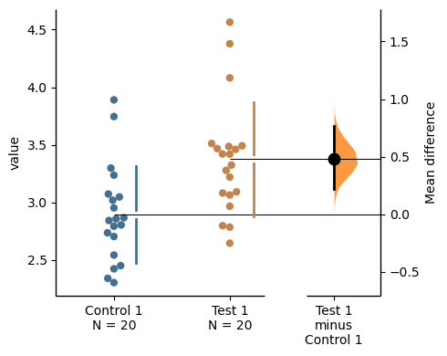
two_groups_unpaired.hedges_g.plot();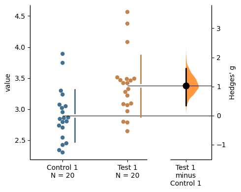
Instead of a Gardner-Altman plot, you can produce a Cumming estimation plot by setting float_contrast=False in the plot() method. This will plot the bootstrap effect sizes below the raw data, and also displays the the mean (gap) and ± standard deviation of each group (vertical ends) as gapped lines. This design was inspired by Edward Tufte’s dictum to maximise the data-ink ratio.
two_groups_unpaired.hedges_g.plot(float_contrast=False);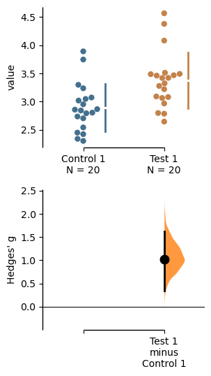
The dabest package also implements a range of estimation plot designs aimed at depicting common experimental designs.
The multi-two-group estimation plot tiles two or more Cumming plots horizontally, and is created by passing a nested tuple to idx when dabest.load() is first invoked.
Thus, the lower axes in the Cumming plot is effectively a forest plot, used in meta-analyses to aggregate and compare data from different experiments.
multi_2group = dabest.load(df, idx=(("Control 1", "Test 1",),
                                         ("Control 2", "Test 2")
                                       ))

multi_2group.mean_diff.plot();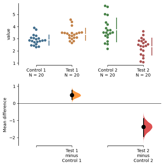
The shared control plot displays another common experimental paradigm, where several test samples are compared against a common reference sample.
This type of Cumming plot is automatically generated if the tuple passed to idx has more than two data columns.
shared_control = dabest.load(df, idx=("Control 1", "Test 1",
                                          "Test 2", "Test 3",
                                          "Test 4", "Test 5", "Test 6")
)shared_controlDABEST v2023.02.14
==================
Good evening!
The current time is Sun Mar 19 22:36:43 2023.
Effect size(s) with 95% confidence intervals will be computed for:
1. Test 1 minus Control 1
2. Test 2 minus Control 1
3. Test 3 minus Control 1
4. Test 4 minus Control 1
5. Test 5 minus Control 1
6. Test 6 minus Control 1
5000 resamples will be used to generate the effect size bootstraps.shared_control.mean_diffDABEST v2023.02.14
==================
Good evening!
The current time is Sun Mar 19 22:36:48 2023.
The unpaired mean difference between Control 1 and Test 1 is 0.48 [95%CI 0.221, 0.768].
The p-value of the two-sided permutation t-test is 0.001, calculated for legacy purposes only.
The unpaired mean difference between Control 1 and Test 2 is -0.542 [95%CI -0.914, -0.211].
The p-value of the two-sided permutation t-test is 0.0042, calculated for legacy purposes only.
The unpaired mean difference between Control 1 and Test 3 is 0.174 [95%CI -0.295, 0.628].
The p-value of the two-sided permutation t-test is 0.479, calculated for legacy purposes only.
The unpaired mean difference between Control 1 and Test 4 is 0.79 [95%CI 0.306, 1.31].
The p-value of the two-sided permutation t-test is 0.0042, calculated for legacy purposes only.
The unpaired mean difference between Control 1 and Test 5 is 0.265 [95%CI 0.0137, 0.497].
The p-value of the two-sided permutation t-test is 0.0404, calculated for legacy purposes only.
The unpaired mean difference between Control 1 and Test 6 is 0.288 [95%CI -0.00441, 0.515].
The p-value of the two-sided permutation t-test is 0.0324, calculated for legacy purposes only.
5000 bootstrap samples were taken; the confidence interval is bias-corrected and accelerated.
Any p-value reported is the probability of observing theeffect size (or greater),
assuming the null hypothesis ofzero difference is true.
For each p-value, 5000 reshuffles of the control and test labels were performed.
To get the results of all valid statistical tests, use `.mean_diff.statistical_tests`shared_control.mean_diff.plot();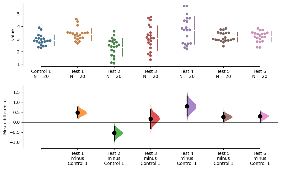
dabest thus empowers you to robustly perform and elegantly present complex visualizations and statistics.
multi_groups = dabest.load(df, idx=(("Control 1", "Test 1",),
                                         ("Control 2", "Test 2","Test 3"),
                                         ("Control 3", "Test 4","Test 5", "Test 6")
))multi_groupsDABEST v2023.02.14
==================
Good evening!
The current time is Sun Mar 19 22:36:56 2023.
Effect size(s) with 95% confidence intervals will be computed for:
1. Test 1 minus Control 1
2. Test 2 minus Control 2
3. Test 3 minus Control 2
4. Test 4 minus Control 3
5. Test 5 minus Control 3
6. Test 6 minus Control 3
5000 resamples will be used to generate the effect size bootstraps.multi_groups.mean_diffDABEST v2023.02.14
==================
Good evening!
The current time is Sun Mar 19 22:37:01 2023.
The unpaired mean difference between Control 1 and Test 1 is 0.48 [95%CI 0.221, 0.768].
The p-value of the two-sided permutation t-test is 0.001, calculated for legacy purposes only.
The unpaired mean difference between Control 2 and Test 2 is -1.38 [95%CI -1.93, -0.895].
The p-value of the two-sided permutation t-test is 0.0, calculated for legacy purposes only.
The unpaired mean difference between Control 2 and Test 3 is -0.666 [95%CI -1.3, -0.103].
The p-value of the two-sided permutation t-test is 0.0352, calculated for legacy purposes only.
The unpaired mean difference between Control 3 and Test 4 is 0.362 [95%CI -0.114, 0.887].
The p-value of the two-sided permutation t-test is 0.161, calculated for legacy purposes only.
The unpaired mean difference between Control 3 and Test 5 is -0.164 [95%CI -0.404, 0.0742].
The p-value of the two-sided permutation t-test is 0.208, calculated for legacy purposes only.
The unpaired mean difference between Control 3 and Test 6 is -0.14 [95%CI -0.398, 0.102].
The p-value of the two-sided permutation t-test is 0.282, calculated for legacy purposes only.
5000 bootstrap samples were taken; the confidence interval is bias-corrected and accelerated.
Any p-value reported is the probability of observing theeffect size (or greater),
assuming the null hypothesis ofzero difference is true.
For each p-value, 5000 reshuffles of the control and test labels were performed.
To get the results of all valid statistical tests, use `.mean_diff.statistical_tests`multi_groups.mean_diff.plot();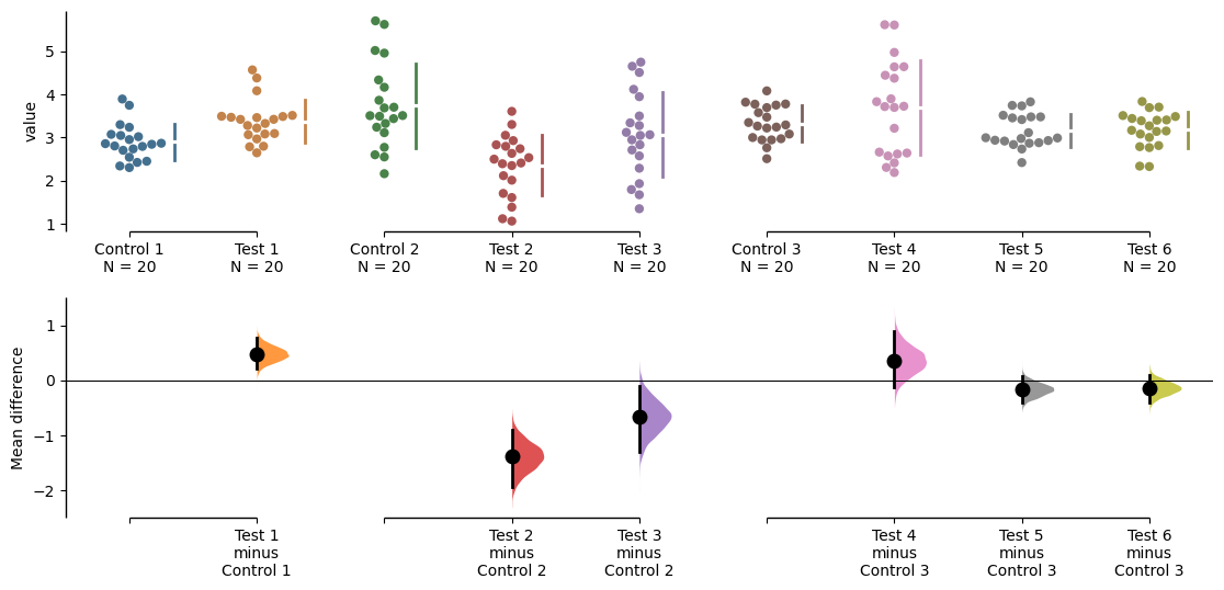
dabest can also work with ‘melted’ or ‘long’ data. This term is so used because each row will now correspond to a single datapoint, with one column carrying the value and other columns carrying ‘metadata’ describing that datapoint.
More details on wide vs long or ‘melted’ data can be found in this Wikipedia article. The pandas documentation gives recipes for melting dataframes.
x='group'
y='metric'

value_cols = df.columns[:-2] # select all but the "Gender" and "ID" columns.

df_melted = pd.melt(df.reset_index(),
                    id_vars=["Gender", "ID"],
                    value_vars=value_cols,
                    value_name=y,
                    var_name=x)

df_melted.head() # Gives the first five rows of `df_melted`.| Gender | ID | group | metric | |
|---|---|---|---|---|
| 0 | Female | 1 | Control 1 | 2.793984 |
| 1 | Female | 2 | Control 1 | 3.236759 |
| 2 | Female | 3 | Control 1 | 3.019149 |
| 3 | Female | 4 | Control 1 | 2.804638 |
| 4 | Female | 5 | Control 1 | 2.858019 |
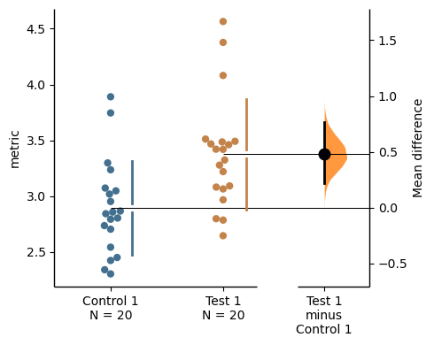
When your data is in this format, you will need to specify the x and y columns in dabest.load().
analysis_of_long_df = dabest.load(df_melted, idx=("Control 1", "Test 1"),
                                     x="group", y="metric")

analysis_of_long_df
DABEST v2023.02.14
==================
Good evening!
The current time is Sun Mar 19 22:37:07 2023.
Effect size(s) with 95% confidence intervals will be computed for:
1. Test 1 minus Control 1
5000 resamples will be used to generate the effect size bootstraps.analysis_of_long_df.mean_diff.plot();