DABEST v2023.2.14
=================
Good evening!
The current time is Fri Mar 31 19:41:17 2023.
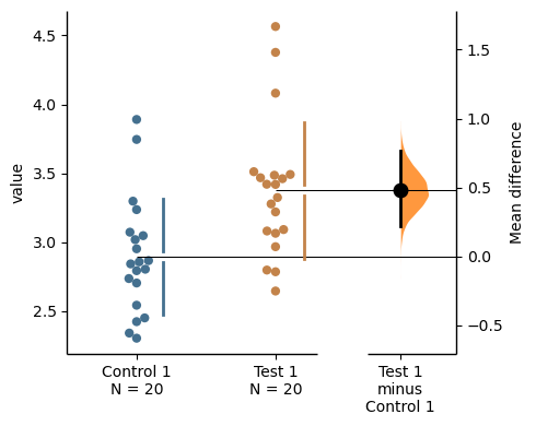
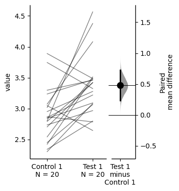
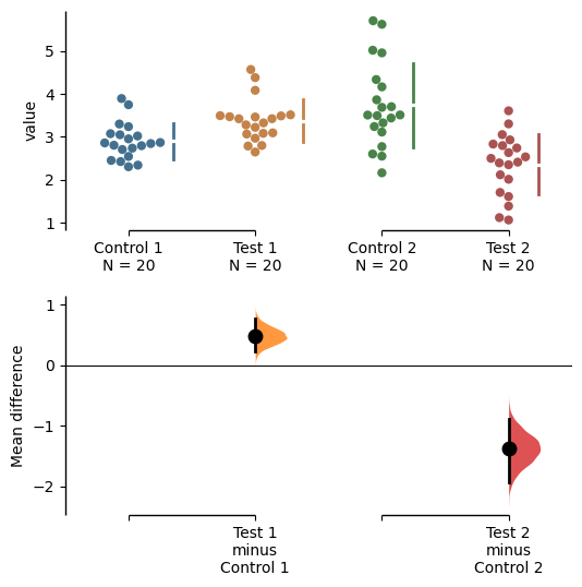
The unpaired mean difference between control and test is 0.5 [95%CI -0.0412, 1.0].
The p-value of the two-sided permutation t-test is 0.0758, calculated for legacy purposes only.
5000 bootstrap samples were taken; the confidence interval is bias-corrected and accelerated.
Any p-value reported is the probability of observing theeffect size (or greater),
assuming the null hypothesis ofzero difference is true.
For each p-value, 5000 reshuffles of the control and test labels were performed.
To get the results of all valid statistical tests, use `.mean_diff.statistical_tests`
This is simply the mean of the control group subtracted from the mean of the test group.
c:\users\zhang\desktop\vnbdev-dabest\dabest-python\dabest\effsize.py:72: UserWarning: Using median as the statistic in bootstrapping may result in a biased estimate and cause problems with BCa confidence intervals. Consider using a different statistic, such as the mean.
When plotting, please consider using percetile confidence intervals by specifying `ci_type='percentile'`. For detailed information, refer to https://github.com/ACCLAB/DABEST-python/issues/129

  return func_difference(control, test, np.median, is_paired)
DABEST v2023.2.14
=================

Good afternoon!
The current time is Thu Mar 30 17:07:33 2023.

The unpaired median difference between control and test is 0.5 [95%CI -0.0758, 0.991].
The p-value of the two-sided permutation t-test is 0.103, calculated for legacy purposes only.

5000 bootstrap samples were taken; the confidence interval is bias-corrected and accelerated.
Any p-value reported is the probability of observing theeffect size (or greater),
assuming the null hypothesis ofzero difference is true.
For each p-value, 5000 reshuffles of the control and test labels were performed.

To get the results of all valid statistical tests, use `.median_diff.statistical_tests`
This is the median difference between the control group and the test group.
If the comparison(s) are unpaired, median_diff is computed with the following equation:
Using median difference as the statistic in bootstrapping may result in a biased estimate and cause problems with BCa confidence intervals. Consider using mean difference instead.
When plotting, consider using percentile confidence intervals instead of BCa confidence intervals by specifying ci_type = 'percentile' in .plot().
For detailed information, please refer to Issue 129.
DABEST v2023.2.14
=================

Good afternoon!
The current time is Thu Mar 30 17:07:39 2023.

The unpaired Cohen's d between control and test is 0.471 [95%CI -0.0843, 0.976].
The p-value of the two-sided permutation t-test is 0.0758, calculated for legacy purposes only.

5000 bootstrap samples were taken; the confidence interval is bias-corrected and accelerated.
Any p-value reported is the probability of observing theeffect size (or greater),
assuming the null hypothesis ofzero difference is true.
For each p-value, 5000 reshuffles of the control and test labels were performed.

To get the results of all valid statistical tests, use `.cohens_d.statistical_tests`
Cohen’s d is simply the mean of the control group subtracted from the mean of the test group.
If paired is None, then the comparison(s) are unpaired; otherwise the comparison(s) are paired.
If the comparison(s) are unpaired, Cohen’s d is computed with the following equation:
\[d = \frac{\overline{x}_{Test} - \overline{x}_{Control}} {\text{pooled standard deviation}}\]
For paired comparisons, Cohen’s d is given by
\[d = \frac{\overline{x}_{Test} - \overline{x}_{Control}} {\text{average standard deviation}}\]
where \(\overline{x}\) is the mean of the respective group of observations, \({Var}_{x}\) denotes the variance of that group,
\[\text{average standard deviation} = \sqrt{ \frac{{Var}_{control} + {Var}_{test}} {2}}\]
The sample variance (and standard deviation) uses N-1 degrees of freedoms. This is an application of Bessel’s correction, and yields the unbiased sample variance.
DABEST v2023.2.14
=================

Good evening!
The current time is Mon Mar 27 00:48:59 2023.

The unpaired Cohen's h between control and test is 0.0 [95%CI -0.613, 0.429].
The p-value of the two-sided permutation t-test is 0.799, calculated for legacy purposes only.

5000 bootstrap samples were taken; the confidence interval is bias-corrected and accelerated.
Any p-value reported is the probability of observing theeffect size (or greater),
assuming the null hypothesis ofzero difference is true.
For each p-value, 5000 reshuffles of the control and test labels were performed.

To get the results of all valid statistical tests, use `.cohens_h.statistical_tests`
Cohen’s h uses the information of proportion in the control and test groups to calculate the distance between two proportions.
It can be used to describe the difference between two proportions as “small”, “medium”, or “large”.
It can be used to determine if the difference between two proportions is “meaningful”.
A directional Cohen’s h is computed with the following equation:
DABEST v2023.2.14
=================
Good evening!
The current time is Mon Mar 27 00:50:18 2023.
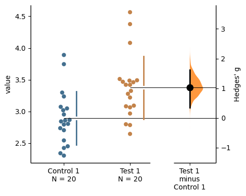
The unpaired Hedges' g between control and test is 0.465 [95%CI -0.0832, 0.963].
The p-value of the two-sided permutation t-test is 0.0758, calculated for legacy purposes only.
5000 bootstrap samples were taken; the confidence interval is bias-corrected and accelerated.
Any p-value reported is the probability of observing theeffect size (or greater),
assuming the null hypothesis ofzero difference is true.
For each p-value, 5000 reshuffles of the control and test labels were performed.
To get the results of all valid statistical tests, use `.hedges_g.statistical_tests`
Hedges’ g is cohens_d corrected for bias via multiplication with the following correction factor:
DABEST v2023.2.14
=================

Good evening!
The current time is Mon Mar 27 00:53:30 2023.

The unpaired Cliff's delta between control and test is 0.28 [95%CI -0.0244, 0.533].
The p-value of the two-sided permutation t-test is 0.061, calculated for legacy purposes only.

5000 bootstrap samples were taken; the confidence interval is bias-corrected and accelerated.
Any p-value reported is the probability of observing theeffect size (or greater),
assuming the null hypothesis ofzero difference is true.
For each p-value, 5000 reshuffles of the control and test labels were performed.

To get the results of all valid statistical tests, use `.cliffs_delta.statistical_tests`
Cliff’s delta is a measure of ordinal dominance, ie. how often the values from the test sample are larger than values from the control sample.
where \(\#\) denotes the number of times a value from the test sample exceeds (or is lesser than) values in the control sample.
Cliff’s delta ranges from -1 to 1; it can also be thought of as a measure of the degree of overlap between the two samples. An attractive aspect of this effect size is that it does not make an assumptions about the underlying distributions that the samples were drawn from.
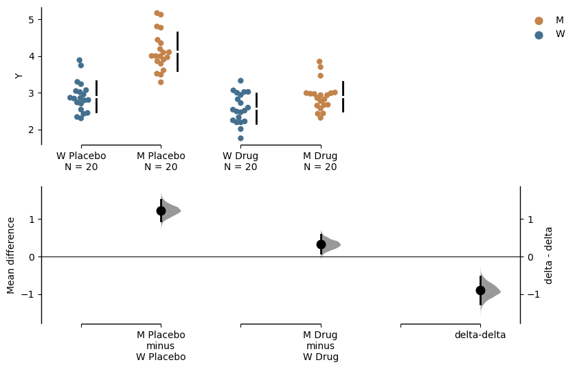
A class to compute and store the delta-delta statistics for experiments with a 2-by-2 arrangement where two independent variables, A and B, each have two categorical values, 1 and 2. The data is divided into two pairs of two groups, and a primary delta is first calculated as the mean difference between each of the pairs:
where \(s\) is the standard deviation and \(n\) is the sample size.
Example: delta-delta
np.random.seed(9999) # Fix the seed so the results are replicable.N =20# Create samplesy = norm.rvs(loc=3, scale=0.4, size=N*4)y[N:2*N] = y[N:2*N]+1y[2*N:3*N] = y[2*N:3*N]-0.5# Add a `Treatment` columnt1 = np.repeat('Placebo', N*2).tolist()t2 = np.repeat('Drug', N*2).tolist()treatment = t1 + t2 # Add a `Rep` column as the first variable for the 2 replicates of experiments donerep = []for i inrange(N*2): rep.append('Rep1') rep.append('Rep2')# Add a `Genotype` column as the second variablewt = np.repeat('W', N).tolist()mt = np.repeat('M', N).tolist()wt2 = np.repeat('W', N).tolist()mt2 = np.repeat('M', N).tolist()genotype = wt + mt + wt2 + mt2# Add an `id` column for paired data plotting.id=list(range(0, N*2))id_col =id+id# Combine all columns into a DataFrame.df_delta2 = pd.DataFrame({'ID' : id_col,'Rep' : rep,'Genotype' : genotype, 'Treatment': treatment,'Y' : y })unpaired_delta2 = dabest.load(data = df_delta2, x = ["Genotype", "Genotype"], y ="Y", delta2 =True, experiment ="Treatment")unpaired_delta2.mean_diff.plot();
DABEST v2023.2.14
=================

Good morning!
The current time is Mon Mar 27 01:01:11 2023.

The weighted-average unpaired mean differences is 0.0336 [95%CI -0.137, 0.228].
The p-value of the two-sided permutation t-test is 0.736, calculated for legacy purposes only.

5000 bootstrap samples were taken; the confidence interval is bias-corrected and accelerated.
Any p-value reported is the probability of observing theeffect size (or greater),
assuming the null hypothesis ofzero difference is true.
For each p-value, 5000 reshuffles of the control and test labels were performed.
As of version 2023.02.14, weighted delta can only be calculated for mean difference, and not for standardized measures such as Cohen’s d.
Details about the calculated weighted delta are accessed as attributes of the mini_meta_delta class. See the minimetadelta for details on usage.
Refer to Chapter 10 of the Cochrane handbook for further information on meta-analysis: https://training.cochrane.org/handbook/current/chapter-10
A class to compute and store the results of bootstrapped mean differences between two groups.
Compute the effect size between two groups.
Type
Default
Details
control
array-like
test
array-like
These should be numerical iterables.
effect_size
string.
Any one of the following are accepted inputs: ‘mean_diff’, ‘median_diff’, ‘cohens_d’, ‘hedges_g’, or ‘cliffs_delta’
proportional
bool
False
is_paired
NoneType
None
ci
int
95
The confidence interval width. The default of 95 produces 95% confidence intervals.
resamples
int
5000
The number of bootstrap resamples to be taken for the calculation of the confidence interval limits.
permutation_count
int
5000
The number of permutations (reshuffles) to perform for the computation of the permutation p-value
random_seed
int
12345
random_seed is used to seed the random number generator during bootstrap resampling. This ensures that the confidence intervals reported are replicable.
Returns
py:class:TwoGroupEffectSize object:
difference : float The effect size of the difference between the control and the test. effect_size : string The type of effect size reported. is_paired : string The type of repeated-measures experiment. ci : float Returns the width of the confidence interval, in percent. alpha : float Returns the significance level of the statistical test as a float between 0 and 1. resamples : int The number of resamples performed during the bootstrap procedure. bootstraps : numpy ndarray The generated bootstraps of the effect size. random_seed : int The number used to initialise the numpy random seed generator, ie.seed_value from numpy.random.seed(seed_value) is returned. bca_low, bca_high : float The bias-corrected and accelerated confidence interval lower limit and upper limits, respectively. pct_low, pct_high : float The percentile confidence interval lower limit and upper limits, respectively.
The unpaired mean difference is -0.253 [95%CI -0.78, 0.25].
The p-value of the two-sided permutation t-test is 0.348, calculated for legacy purposes only.

5000 bootstrap samples were taken; the confidence interval is bias-corrected and accelerated.
Any p-value reported is the probability of observing theeffect size (or greater),
assuming the null hypothesis ofzero difference is true.
For each p-value, 5000 reshuffles of the control and test labels were performed.
Any one of the following are accepted inputs: ‘mean_diff’, ‘median_diff’, ‘cohens_d’, ‘hedges_g’, or ‘cliffs_delta’
is_paired
str
None
permutation_count
int
5000
The number of permutations (reshuffles) to perform.
random_seed
int
12345
random_seed is used to seed the random number generator during bootstrap resampling. This ensures that the generated permutations are replicable.
kwargs
Returns
py:class:PermutationTest object:
difference:float The effect size of the difference between the control and the test. effect_size:string The type of effect size reported.
Notes:
The basic concept of permutation tests is the same as that behind bootstrapping. In an “exact” permutation test, all possible resuffles of the control and test labels are performed, and the proportion of effect sizes that equal or exceed the observed effect size is computed. This is the probability, under the null hypothesis of zero difference between test and control groups, of observing the effect size: the p-value of the Student’s t-test.
Exact permutation tests are impractical: computing the effect sizes for all reshuffles quickly exceeds trivial computational loads. A control group and a test group both with 10 observations each would have a total of \(20!\) or \(2.43 \times {10}^{18}\) reshuffles. Therefore, in practice, “approximate” permutation tests are performed, where a sufficient number of reshuffles are performed (5,000 or 10,000), from which the p-value is computed.